RF Simulation
Warning
This page could still use more content! Contributions are welcome.
If you are willing to contribute documentation, please see GitHub issue #23.
Qucs-S also supports a number of simulation devices and techniques that are tailored to RF and microwave (high-frequency) simulation. The specific features available depend on which simulation backend you have selected - see the sections below for more details.
Qucs-S also provides a number of diagrams which are especially useful for microwave and RF circuits. These include:
Smith Chart
Admittance Smith Chart
Polar Complex Plane
Combined Smith Chart and Complex Plane
S-Parameter Simulation with ngspice
Warning
ngspice introduced S-Parameter Simulation in Version 37 (released mid-2022). Make sure your ngspice backend is Version 37 or later, or you will not be able to take advantage of these features!
S-Parameters (Scattering Parameters) are a commonly used tool in high-frequency circuit analysis. For a brief introduction to S-Parameters, see this video (no affiliation to the Qucs-S project)..
Setting up the circuit
To use S-Parameter simulation, you must place two special components on your schematic:
The “S-Parameter Simulation” simulation component. This tells Qucs-S that you wish to perform an S-Parameter simulation. Note that this is the same component used in S-Parameter simulations with Qucsator, although that is where the similarities end.
The “Power Source” component. This is the special RF source that will be used to test and obtain the S-Parameters of your circuit.
Examples of each component, and its properties, are shown in the figures below.
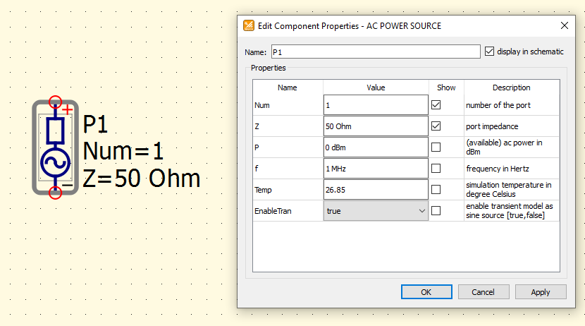
Example of the Power Source component, for use with ngspice when performing S-Parameter Simulations.
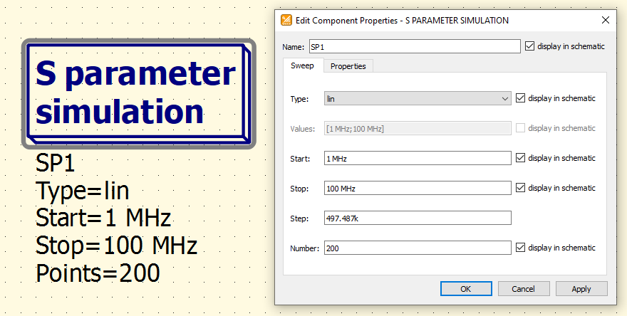
Example of the S-Parameter Simulation component.
As an example, we’ll simulate the frequency response of a bandpass filter for the 20-meter band (part of the amateur radio spectrum). The figure below shows the circuit, and the resulting output graphs.
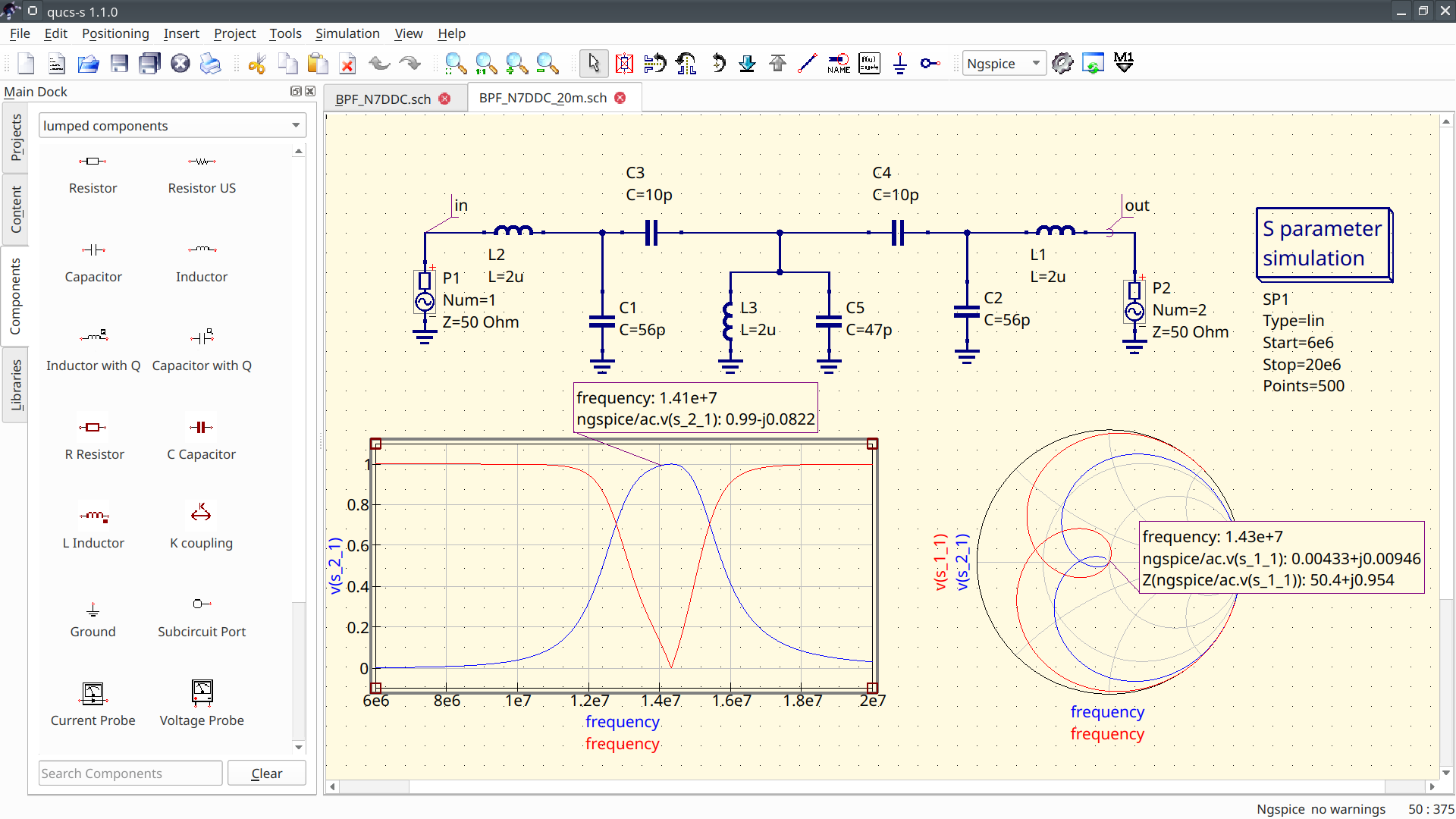
Example of a bandpass filter (designed for the 20-meter amateur radio band), utilizing the ngspice S-Parameter Simulation feature.
The filter itself is made up of LC devices, and the schematic also contains two Power Source components to stimulate the filter. One is connected to the input node (labeled in), and the other is connected to the output node (labeled out).
Finally, the S-Parameter Simulation component defines the frequency sweep range: 6MHz to 20MHz.
Accessing S-Parameter Outputs from ngspice
After running the simulation, the S-Parameter data can be plotted by referencing special “voltages” that ngspice provides in the simulation output. For example, to plot the \(S_{21}\) parameter, you’d need to plot the v(s_2_1) variable.
ngspice also converts the S-Parameters to Y and Z parameters automatically. The Y and Z parameters are also available via special “voltage” variables, in the same syntax as the S parameters. For example, to plot \(Y_{11}\), you should select v(y_1_1).
RF/Transmission Line Simulation with QucsatorRF
While the QucsatorRF simulation backend is very poorly suited for general-purpose time-domain circuit simulation, it is very well suited for RF simulation, particularly in the frequency domain. It has a number of special features that make it a great choice for simulating RF and microwave systems, particularly those involving transmission lines.
Tip
QucsatorRF has been shipped with the main Qucs-S application since version v24.2.0. No manual installation of QucsatorRF is necessary.
For more information on QucsatorRF and the other simulation backends, see the page on simulation backends.
QucsatorRF supports advanced RF simulation techniques, such as multi-port S-Parameter simulation (including 1-port), and harmonic balance (HB) analysis.
QucsatorRF also includes a number of transmission line models, allowing you to model particular geometries on particular substrates. While these models are not full 3D field solvers, they are significantly more detailed and customizable than the transmission line models included with other backends, such as ngspice.
The most commonly used QucsatorRF transmission line models are:
4-Terminal Transmission Line
Twisted Pair
Coaxial Cable
Microstrip Lines (including special components for modeling tees and corners)
Coupled Microstrips
Coplanar Lines
Waveguides
Generic RLCG Line (distributed-element lines, the model used by the telegrapher’s equations)
Using Transmission Line Models with QucsatorRF
Warning
If you are having trouble finding the components referenced in this section, be sure that QucsatorRF is selected as your simulation backend. Qucs-S will only show components that are compatible with the currently-selected simulation backend. See the Interface Overview page for details on how to adjust this setting.
To use any of the transmission line models with QucsatorRF, you must first place a Substrate component on the schematic page. This defines the material properties. Each substrate is assigned an identifier (for example, Substr1), so you can use multiple substrates on a single schematic page, to model more complex multi-material systems.
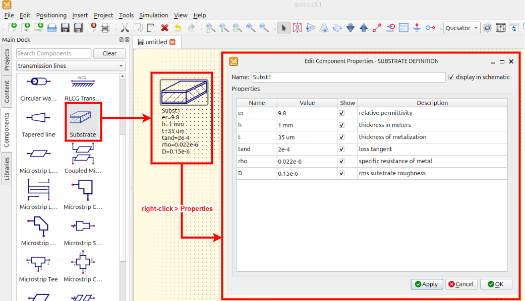
Example of the Substrate component, used to specify material properties of a transmission line component.
After placing at least one Substrate component, transmission line components can be placed on the schematic page, referencing the substrate for their material properties. Simply type in the ID of the substrate (for example, Substr1) as the value for the Substr parameter on your transmission line.
Example
As an example, the figure below shows a 1.5GHz coupled microstrip band-pass filter. It has two ports (Power Source devices P1 and P2) connected to input and output, and two microstrip devices (MS1 and MS2), bound to a substrate (Substr1). Finally, the S-Parameter Simulation component defines the simulation type, and frequency range.
Tip
Although QucsatorRF supports different transmission line models than ngspice, the S-Parameter Simulation component is the same across both backends.
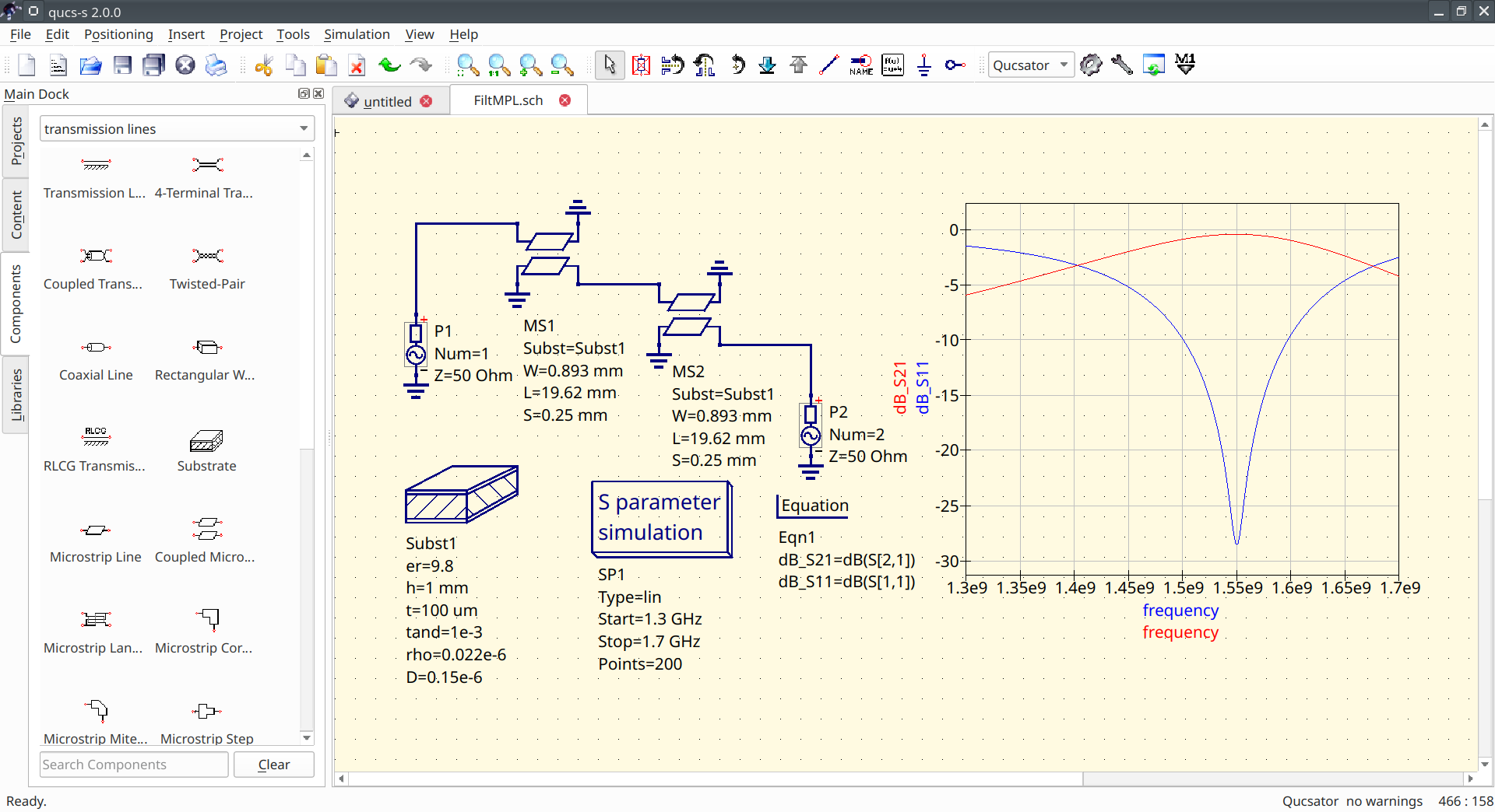
Example of a 1.5GHz coupled microstrip band-pass filter, being simulated with QucsatorRF. It has two ports (Power Source devices P1 and P2) connected to input and output, and two microstrip devices (MS1 and MS2), bound to a substrate (Substr1). Finally, the S-Parameter Simulation component defines the simulation type, and frequency range.
Accessing Results
There are a few key differences in how results are accessed in QucsatorRF, compared to other backends like ngspice:
The equation syntax for QucsatorRF is different, and not cross-compatible with ngspice.
In QucsatorRF, the S-parameters are represented in
S[i,j]form. For example,S[2,1]for \(S_{21}\).In QucsatorRF, Y and Z matrices are NOT calculated automatically (unlike ngspice). If you want these matrices, you’ll need to use the
stoy()andstoz()functions.