Using Equations in QucsatorRF¶

Like ngspice, QucsatorRF also has an Equations feature.

However, unlike ngspice, QucsatorRF does not separate things into Parameters and Equations based on when they are computed. In QucsatorRF, all variables/data are accessible from the Equations feature. There is no need to use a different feature for pre-simulation and post-simulation computations.

The QucsatorRF Equations feature is very similar to the Equations feature in the upstream Qucs project. The QucsatorRF simulation backend is a fork of Qucsator, the only simulation backend supported by the upstream Qucs project. This means that most equations written for upstream Qucs will “just work” in Qucs-S, when used with QucsatorRF as the backend.

Example: RC Filter¶

When showing how to utilize Parameters and Equations in ngspice, an RC filter was used an example circuit. In that example, Parameters were used to manipulate component values before the simulation, while Equations were used to manipulate the results for graphing.

With QucsatorRF, the pre-processing and post-processing features are combined into a single Equations feature. This is accessible via the Qucsator Equation component, as shown below.

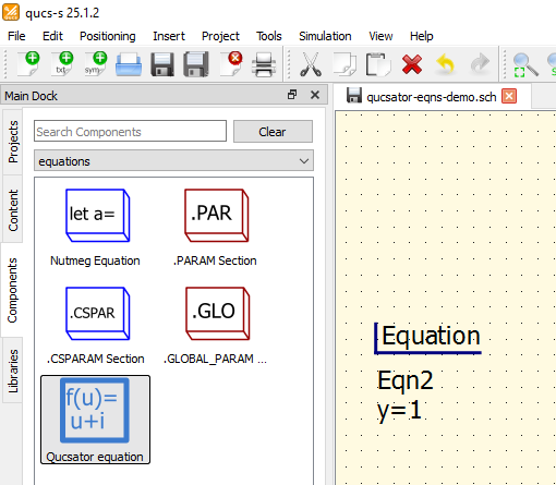
../../_images/qucsator-equation-component.png — The *Qucsator Equation* schematic component, shown in the component browser at left, and placed on the schematic page at right.¶

To demonstrate this, we’ll use the same RC filter as the ngspice example. In Qucsator, it’s possible to create a single Equation component containing both the design equations (governing component values) and the postprocessing equation (the ratio of output to input voltage). The text of this equation is shown below (note the syntax difference in QucsatorRF equations compared to ngspice Nutmeg Equations and Parameters).

Warning

Qucsator equations are case-sensitive! This includes references to built-in functions.

For example, db(foo) will not work, you need to call dB(foo) instead.

r_1 = 1k
fc = 2k
C = 1/(2*pi*fc*r_1)
ratio_linear = out.v/in.v
ratio_dB = dB(out.v/in.v)

Using the equation text from above, we can create the following circuit. Note the graphed results contain both dB and linear format, utilizing the dB() function in QucsatorRF to easily produce a graph in dB format.

../../_images/qucsator-eqns-demo.png — An example circuit utilizing the *Equations* feature with Qucsator.¶

Additional Examples¶

Since the syntax has remained unchanged since Qucs v0.0.19, many of the tutorials for original Qucs still apply to Qucsator Equations in Qucs-S. For additional examples, you may wish to visit these references:

Syntax Basics¶

The following operations and functions can be applied in QucsatorRF equations. Parameters in brackets [...] are optional.

Tip

For a more exhaustive reference, please see the Measurement Expressions Reference Manual, a document written by the original Qucs team. The syntax for QucsatorRF equations in Qucs-S is unchanged compared to upstream Qucs.

Operators¶

Arithmetic Operators¶


`+x`	Unary plus
`-x`	Unary minus
`x+y`	Addition
`x-y`	Subtraction
`x*y`	Multiplication
`x/y`	Division
`x%y`	Modulo (remainder of division)
`x^y`	Power

Logical Operators¶


`!x`	Negation
`x&&y`	And
`x
`x^^y`	Exclusive or
`x?y:z`	Abbreviation for conditional expression - if `x` then `y` else `z`
`x==y`	Equal
`x!=y`	Not equal
`x<y`	Less than
`x<=y`	Less than or equal
`x>y`	Larger than
`x>=y`	Larger than or equal

Math Functions¶

Vectors and Matrices: Creation¶


`eye(n)`	Creates `n` x `n` identity matrix
`length(y)`	Returns the length of the `y` vector
`linspace(from,to,n)`	Real vector with `n` lin spaced components between `from` and `to`
`logspace(from,to,n)`	Real vector with `n` log spaced components between `from` and `to`

Vectors and Matrices: Basic Matrix Functions¶


`adjoint(x)`	Adjoint matrix of `x` (transposed and conjugate complex)
`det(x)`	Determinant of a matrix `x`
`inverse(x)`	Inverse matrix of `x`
`transpose(x)`	Transposed matrix of `x` (rows and columns exchanged)

Elementary Mathematical Functions: Basic Real and Complex Functions¶


`abs(x)`	Absolute value, magnitude of complex number
`angle(x)`	Phase angle in radians of a complex number. Synonym for `arg()`
`arg(x)`	Phase angle in radians of a complex number
`conj(x)`	Conjugate of a complex number
`deg2rad(x)`	Converts phase from degrees into radians
`hypot(x,y)`	Euclidean distance function
`imag(x)`	Imaginary part of a complex number
`mag(x)`	Magnitude of a complex number
`norm(x)`	Square of the absolute value of a vector
`phase(x)`	Phase angle in degrees of a complex number
`polar(m,p)`	Transform polar coordinates `m` and `p` into a complex number
`rad2deg(x)`	Converts phase from radians into degrees
`real(x)`	Real part of a complex number
`sign(x)`	Signum function
`sqr(x)`	Square (power of two) of a number
`sqrt(x)`	Square root
`unwrap(p[,tol[,step]])`	Unwrap angle `p` (radians) – defaults `step` = 2pi, `tol` = pi

Elementary Mathematical Functions: Exponential and Logarithmic Functions¶


`exp(x)`	Exponential function to basis e
`limexp(x)`	Limited exponential function
`log10(x)`	Decimal logarithm
`log2(x)`	Binary logarithm
`ln(x)`	Natural logarithm (base e )

Elementary Mathematical Functions: Trigonometry¶


`cos(x)`	Cosine function
`cosec(x)`	Cosecant
`cot(x)`	Cotangent function
`sec(x)`	Secant
`sin(x)`	Sine function
`tan(x)`	Tangent function

Elementary Mathematical Functions: Inverse Trigonometric Functions¶


`arccos(x)`	Arc cosine (also known as “inverse cosine”)
`arccosec(x)`	Arc cosecant
`arccot(x)`	Arc cotangent
`arcsec(x)`	Arc secant
`arcsin(x)`	Arc sine (also known as “inverse sine”)
`arctan(x[,y])`	Arc tangent (also known as “inverse tangent”)

Elementary Mathematical Functions: Hyperbolic Functions¶


`cosh(x)`	Hyperbolic cosine
`cosech(x)`	Hyperbolic cosecant
`coth(x)`	Hyperbolic cotangent
`sech(x)`	Hyperbolic secant
`sinh(x)`	Hyperbolic sine
`tanh(x)`	Hyperbolic tangent

Elementary Mathematical Functions: Inverse Hyperbolic Functions¶


`arcosh(x)`	Hyperbolic area cosine
`arcosech(x)`	Hyperbolic area cosecant
`arcoth(x)`	Hyperbolic area cotangent
`arsech(x)`	Hyperbolic area secant
`arsinh(x)`	Hyperbolic area sine
`artanh(x)`	Hyperbolic area tangent

Elementary Mathematical Functions: Rounding¶


`ceil(x)`	Round to the next higher integer
`fix(x)`	Truncate decimal places from real number
`floor(x)`	Round to the next lower integer
`round(x)`	Round to nearest integer

Elementary Mathematical Functions: Special Mathematical Functions¶


`besseli0(x)`	Modified Bessel function of order zero
`besselj(n,x)`	Bessel function of first kind and `n`-th order
`bessely(n,x)`	Bessel function of second kind and `n`-th order
`erf(x)`	Error function
`erfc(x)`	Complementary error function
`erfinv(x)`	Inverse error function
`erfcinv(x)`	Inverse complementary error function
`sinc(x)`	Sinc function (sin(`x`)/`x` or 1 at `x` = 0)
`step(x)`	Step function

Data Analysis: Basic Statistics¶


`avg(x[,range])`	Average of vector `x`. If range given `x` must have a single data dependency
`cumavg(x)`	Cumulative average of vector elements
`max(x,y)`	Returns the greater of the values `x` and `y`
`max(x[,range])`	Maximum of vector `x`. If range given `x` must have a single data dependency
`min(x,y)`	Returns the lesser of the values `x` and `y`
`min(x[,range])`	Minimum of vector `x`. If range is given `x` must have a single data dependency
`rms(x)`	Root Mean Square of vector elements
`runavg(x)`	Running average of vector elements
`stddev(x)`	Standard deviation of vector elements
`variance(x)`	Variance of vector elements
`random()`	Random number between 0.0 and 1.0
`srandom(x)`	Give random seed

Data Analysis: Basic Operation¶

`cumprod(x)`	Cumulative product of vector elements
`cumsum(x)`	Cumulative sum of vector elements
`interpolate(f,x[,n])`	Spline interpolation of vector `f` using `n` equidistant points of `x`
`prod(x)`	Product of vector elements
`sum(x)`	Sum of vector elements
`xvalue(f,yval)`	Returns x-value nearest to `yval` in single dependency vector `f`
`yvalue(f,xval)`	Returns y-value nearest to `xval` in single dependency vector `f`

Data Analysis: Differentiation and Integration¶


`ddx(expr,var)`	Derives mathematical expression `expr` with respect to the variable `var`
`diff(y,x[,n])`	Differentiate vector `y` with respect to vector `x` `n` times. Defaults to `n` = 1
`integrate(x,h)`	Integrate vector `x` numerically assuming a constant step-size `h`

Data Analysis: Signal Processing¶


`dft(x)`	Discrete Fourier Transform of vector `x`
`fft(x)`	Fast Fourier Transform of vector `x`
`fftshift(x)`	Shuffles the FFT values of vector `x` to move DC to the center of the vector
`Freq2Time(V,f)`	Inverse Discrete Fourier Transform of function `V(f)` interpreting it physically
`idft(x)`	Inverse Discrete Fourier Transform of vector `x`
`ifft(x)`	Inverse Fast Fourier Transform of vector `x`
`kbd(x[,n])`	Kaiser-Bessel derived window
`Time2Freq(v,t)`	Discrete Fourier Transform of function `v(t)` interpreting it physically

Electronics Functions¶

Unit Conversion¶


`dB(x)`	dB value
`dbm(x)`	Convert voltage to power in dBm
`dbm2w(x)`	Convert power in dBm to power in Watts
`w2dbm(x)`	Convert power in Watts to power in dBm
`vt(t)`	Thermal voltage for a given temperature `t` in Kelvin

Reflection Coefficients and VSWR¶


`rtoswr(x)`	Converts reflection coefficient to voltage standing wave ratio (VSWR)
`rtoy(x[,zref])`	Converts reflection coefficient to admittance; default `zref` = 50 ohms
`rtoz(x[,zref])`	Converts reflection coefficient to impedance; default `zref` = 50 ohms
`ytor(x[,zref])`	Converts admittance to reflection coefficient; default `zref` = 50 ohms
`ztor(x[,zref])`	Converts impedance to reflection coefficient; default `zref` = 50 ohms

N-Port Matrix Conversions¶


`stos(s,zref[,z0])`	Converts S-parameter matrix to S-parameter matrix with a different Z0
`stoy(s[,zref])`	Converts S-parameter matrix to Y-parameter matrix
`stoz(s[,zref])`	Converts S-parameter matrix to Z-parameter matrix
`twoport(m,from,to)`	Converts a two-port matrix: `from` and `to` are ‘Y’, ‘Z’, ‘H’, ‘G’, ‘A’, ‘S’ and ‘T’.
`ytos(y[,z0])`	Converts Y-parameter matrix to S-parameter matrix
`ytoz(y)`	Converts Y-parameter matrix to Z-parameter matrix
`ztos(z[,z0])`	Converts Z-parameter matrix to S-parameter matrix
`ztoy(z)`	Converts Z-parameter matrix to Y-parameter matrix

Amplifiers¶


`GaCircle(s,Ga[,arcs])`	Available power gain `Ga` circles (source plane )
`GpCircle(s,Gp[,arcs])`	Operating power gain `Gp` circles (load plane)
`Mu(s)`	Mu stability factor of a two-port S-parameter matrix
`Mu2(s)`	Mu’ stability factor of a two-port S-parameter matrix
`NoiseCircle(Sopt,Fmin,Rn,F[,Arcs])`	Noise Figure(s) `F` circles
`PlotVs(data,dep)`	Returns data selected from `data`: dependency `dep`
`Rollet(s)`	Rollet stability factor of a two-port S-parameter matrix
`StabCircleL(s[,arcs])`	Stability circle in the load plane
`StabCircleS(s[,arcs])`	Stability circle in the source plane
`StabFactor(s)`	Stability factor of a two-port S-parameter matrix
`StabMeasure(s)`	Stability measure B1 of a two-port S-parameter matrix

Nomenclature¶

Ranges¶


`LO:HI`	Range from `LO` to `HI`
`:HI`	Up to `HI`
`LO:`	From `LO`
`:`	No range limitations

Matrices and Matrix Elements¶


`M`	The whole matrix `M`
`M[2,3]`	Element being in 2nd row and 3rd column of matrix `M`
`M[:,3]`	Vector consisting of 3rd column of matrix `M`

Immediate¶


`2.5`	Real number
`1.4+j5.1`	Complex number
`[1,3,5,7]`	Vector
`[11,12;21,22]`	Matrix

Number suffixes¶


`E`	exa, 1e+18
`P`	peta, 1e+15
`T`	tera, 1e+12
`G`	giga, 1e+9
`M`	mega, 1e+6
`k`	kilo, 1e+3
`m`	milli, 1e-3
`u`	micro, 1e-6
`n`	nano, 1e-9
`p`	pico, 1e-12
`f`	femto, 1e-15
`a`	atto, 1e-18

Name of Values¶


`S[1,1]`	S-parameter value
nodename.`V`	DC voltage at node nodename
name.`I`	DC current through component name
nodename.`v`	AC voltage at node nodename
name.`i`	AC current through component name
nodename.`vn`	AC noise voltage at node nodename
name.`in`	AC noise current through component name
nodename.`Vt`	Transient voltage at node nodename
name.`It`	Transient current through component name

Note: All voltages and currents are peak values. Note: Noise voltages are RMS values at 1 Hz bandwidth.

Constants¶


`i, j`	Imaginary unit (“square root of -1”)
`pi`	4*arctan(1) = 3.14159…
`e`	Euler = 2.71828…
`kB`	Boltzmann constant = 1.38065e-23 J/K
`q`	Elementary charge = 1.6021765e-19 C

Equations & Parameters with ngspice

Displaying Results