Equations & Parameters with ngspice

Equations vs Parameters

ngspice has two complementary features:

• Parameters are computed BEFORE your simulation executes. They can be used to manipulate component values or other circuit properties. This uses the SPICE .PARAM feature.

• Equations are computed AFTER your simulation is complete. They can be used to manipulate the results of your simulation, for graphing or further analysis.

The diagram below shows where Parameters and Equations each fit into the Simulation process.

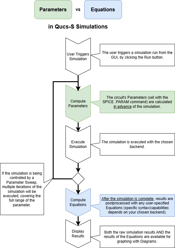
A simplified diagram of the steps in the Qucs-S simulation process, highlighting the times where Parameters and Equations are computed.

Parameters in ngspice with .PARAM

The Parameters feature can be used much like the Parametric Design features in many mechanical CAD packages. It allows you to describe your circuit elements using parameters, instead of being limited to “hardcoded” constant values. When you run your simulation, these Parameters will be computed BEFORE the simulation actually executes.

Parameter Syntax Basics

The .PARAM syntax is mostly common across all SPICE-compatible simulation engines.

For a definitive reference, see the ngspice manual.

You may also find the LTSpice Wiki helpful as a quick reference.

Operators

Operators available in SPICE .PARAM statements, with their “precedence” in the order of operations listed as well. Taken from the ngspice manual.

Operator	Alias	Precedence	Description
-		1	unary -
!		1	unary not
**	^	2	power, like pwr
*		3	multiply
/		3	divide
%		3	modulo
\		3	integer divide
+		4	add
-		4	subtract
==		5	equality
!=	<>	5	non-equal
<=		5	less or equal
>=		5	greater or equal
<		5	less than
>		5	greater than
&&		6	boolean and
||		7	boolean or
c?x:y		8	ternary operator

Functions

A list of functions available in SPICE .PARAM statements. Taken from the ngspice manual.

Built-in function	Notes
sqrt(x)	y = sqrt(x)
sin(x), cos(x), tan(x)
sinh(x), cosh(x), tanh(x)
asin(x), acos(x), atan(x)
asinh(x), acosh(x), atanh(x)
arctan(x)	atan(x), kept for compatibility
exp(x)
ln(x), log(x)
abs(x)
nint(x)	Nearest integer, half integers towards even
int(x)	Nearest integer rounded towards 0
floor(x)	Nearest integer rounded towards -∞
ceil(x)	Nearest integer rounded towards +∞
pow(x,y)	x raised to the power of y (pow from C runtime library)
pwr(x,y)	pow(fabs(x), y)
min(x, y)
max(x, y)
sgn(x)	1.0 for x > 0, 0.0 for x == 0, -1.0 for x < 0
ternary_fcn(x, y, z)	x ? y : z
gauss(nom, rvar, sigma)	nominal value plus variation drawn from Gaussian distribution with mean 0 and standard deviation rvar (relative to nominal), divided by sigma
agauss(nom, avar, sigma)	nominal value plus variation drawn from Gaussian distribution with mean 0 and standard deviation avar (absolute), divided by sigma
unif(nom, rvar)	nominal value plus relative variation (to nominal) uniformly distributed between +/-rvar
aunif(nom, avar)	nominal value plus absolute variation uniformly distributed between +/-avar
limit(nom, avar)	nominal value +/-avar, depending on random number in [-1, 1[ being > 0 or < 0

Scaling Suffixes

Typical SI Suffixes can be used to scale units. See the table below for syntax.

Built-in keywords for scaling units according to the International System of Units (SI).

Suffix	Name	Value
g	Giga	1e9
meg	Mega	1e6
k	Kilo	1e3
m	Milli	1e-3
u	Micro	1e-6
n	Nano	1e-9
p	Pico	1e-12
f	Femto	1e-15

Example Circuit using Parameters (.PARAM)

Consider a simple low-pass filter made up of a resistor and a capacitor. According to the well-known design equations for this type of filter, the half-power cutoff frequency can be described with the equation below:

\(f_{c}=\frac{1}{2\pi RC}\)

With some algebra, we can define \(C\) in terms of \(f_{c}\) and \(R\):

\(C=\frac{1}{2\pi f_{c} R}\)

At this point, we can use the Parameters feature to calculate the value of C for a given cutoff frequency automatically.

Tip

If you need to use Pi (\(\pi\)) in a SPICE .PARAM component, use the following code: pi={4*atan(1)}

After adding the code to create the constant Pi, and adding the design equation from above, we arrive at this .PARAM code (with desired cutoff frequency set to 2kHz):

R = 1k
fc = 2k
pi = {4*atan(1)}
C = (1)/(2*pi*fc*R)

After building up the rest of the filter circuit using an AC Simulation, we can see the result is a success:

Example using the Parameters (.PARAM) feature, to automatically calculate the capacitor value in an RC Low-Pass filter based on a desired cutoff frequency.

Equations in ngspice with Nutmeg

In contrast to the Parameters feature from the previous section, Equations are calculated AFTER your simulation is complete. They are useful for analyzing results, and manipulating your simulation data for display on a Diagram (graph).

When using ngspice, Qucs-S leverages its built in “Nutmeg” postprocessor system for an “Equations” functionality.

Warning

Note that Nutmeg is NOT the same as the recently-deprecated ngnutmeg command-line utility. The ngspice manual mentions several times that ngnutmeg is obsolete, but that does NOT mean that the full Nutmeg functionality is obsolete, and it does not affect the Nutmeg Equation function in Qucs-S.

To use this feature, place a Nutmeg Equation component on your schematic page. You can find this component under the Equations category. An example of the component is shown below, with its Properties dialog annotated.

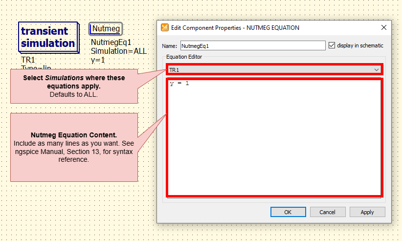
An example of a Nutmeg Equation block, and its Properties. Annotated for clarity.

Tip

You can select which Simulation Components a given Nutmeg Equation block applies to, within the Properties dialog.

By default, Nutmeg Equation blocks apply to all simulations on the schematic page. In most cases, this will suffice. However, in particularly complex simulation cases, limiting the scope to certain simulations may reduce simulation time, or reduce the complexity of the output.

Nutmeg Syntax Basics

Tip

For an exhaustive syntactical reference on ngspice Nutmeg equations, see the ngspice manual, Section 13 “Interactive Interpreter”.

The Nutmeg equation syntax is relatively simple, and supports all the common mathematical operators, as well as many special functions (trigonometric, logarithmic, etc).

First, it’s necessary to understand that ngspice stores all data as a vector. Even scalars are vectors “under the hood”, they simply have a length of 1.

Algebraic Operators

• + : Addition

• - : Subtraction

• * : Multiplication

• / : Division

• ^ : Exponent

• % : Modulo (Remainder)

• , : Dual-purpose operator, depending on context.

  • If it is used in the arguments list of a user-definable function, it separates the arguments (like most programming languages).

  • In all other cases, it serves as a way to express complex numbers/vectors. For example, x , y is synonymous with x + j(y).

Boolean/Relational Operators

• gt : Equivalent to \(>\)

• lt : Equivalent to \(<\)

• ge : Equivalent to \(>=\)

• le : Equivalent to \(<=\)

• ne : Equivalent to \(<>\)

• and : Equivalent to &

• or : Equivalent to \(|\)

• not : Equivalent to \(!\)

• eq : Equivalent to \(=\)

Comments

You can place comments anywhere you like in a Nutmeg Equation. Simply begin the line with ;, and that line will be considered a comment. There is no support for “inline” comments - comments must take an entire line. An example of commenting is shown below.

;This line is a comment, and will be ignored
y=x*log(a)
;The equation above will be parsed normally

Built-In Constants and Variables

ngspice provides a number of pre-defined constants, which you can reference by name. Note that they are all given in MKS units. See table below.

Built-in constants available in ngspice. Taken from the ngspice manual.

Name	Description	Value
pi	π	3.14159…
e	e (the base of natural logarithms)	2.71828…
c	c (the speed of light)	299,792,458 m sec
i	i (the square root of -1)	\(\sqrt -1\)
kelvin	(absolute zero in centigrade)	-273.15 °C
echarge	q (the charge of an electron)	1.60219e-19 C
boltz	k (Boltzmann’s constant)	1.38062e-23 J K
planck	h (Planck’s constant)	6.62607e-34 J s
yes	boolean	1
no	boolean	0
TRUE	boolean	1
FALSE	boolean	0

Functions

Functions provided by ngspice. Taken from the ngspice manual.

Name	Function
mag(vector)	Magnitude of vector (same as abs(vector)).
ph(vector)	Phase of complex vector, in radians.
cph(vector)	Phase of complex vector, in radians. Continuous values, no discontinuity at ± π .
unwrap(vector)	Phase of vector with real phase vector in degrees as input and output. Continuous values, no discontinuity at ±180.
j(vector)	i (sqrt(-1)) times vector.
real(vector)	The real component of vector.
imag(vector)	The imaginary part of vector.
conj(vector)	The complex conjugate of a vector
db(vector)	20 log10(mag(vector)).
log10(vector)	The logarithm (base 10) of vector.
ln(vector)	The natural logarithm (base e) of vector.
exp(vector)	e to the vector power.
abs(vector)	The absolute value of vector (same as mag).
sqrt(vector)	The square root of vector.
sin(vector)	The sine of vector.
cos(vector)	The cosine of vector.
tan(vector)	The tangent of vector.
atan(vector)	The inverse tangent of vector.
sinh(vector)	The hyperbolic sine of vector.
cosh(vector)	The hyperbolic cosine of vector.
tanh(vector)	The hyperbolic tangent of vector.
atanh(vector)	The inverse hyperbolic tangent of vector.
floor(vector)	Largest integer that is less than or equal to vector.
ceil(vector)	Smallest integer that is greater than or equal to vector.
norm(vector)	The vector normalized to 1 (i.e, the largest magnitude of any component is 1).
mean(vector)	The result is a scalar (a length 1 vector) that is the mean of the elements of vector (elements values added, divided by number of elements).
avg(vector)	The average of a vector.Returns a vector where each element is the mean of the preceding elements of the input vector (including the actual element).
stddev(vector)	The result is a scalar (a length 1 vector) that is the standard deviation of the elements of vector .
group_delay(vector)	Calculates the group delay -dphase[ rad ]/dω[ rad/s ] . Input is the complex vector of a system transfer function versus frequency, resembling damping and phase per frequency value. Output is a vector of group delay values (real values of delay times) versus frequency.
vector(number)	The result is a vector of length number, with elements 0, 1, … number - 1. If number is a vector then just the first element is taken, and if it isn’t an integer then the floor of the magnitude is used.
cvector(number)	Return a vector of length number, containing complex elements, with the real part values increasing from 0 to number-1, the imaginary values are set to 0.
unitvec(number)	The result is a vector of length number, all elements having a value 1.
length(vector)	The length of vector.
interpolate(plot.vector)	The result of interpolating the named vector onto the scale of the current plot. This function uses the variable polydegree to determine the degree of interpolation.
integ(vector)	Integrates over the given vector (versus the real component of the scale vector), using the trapeziodal method. The result is another vector, showing the integral up to the current scale value. See also 11.4.8 for measuring the integral sum for a section of a vector, and 8.2.17 for integration on the fly during a transient simulation.
deriv(vector)	Calculates the derivative of the given vector. This uses numeric differentiation by interpolating a polynomial. The degree of the polynomal may be set by the variable dpolydegree (default is 2). The procedure may not produce satisfactory results (particularly with iterated differentiation). The implementation only calculates the derivative with respect to the real component of that vector’s scale.
vecd(vector)	Compute the differential of a vector.
vecmin(vector)	Returns the value of the vector element with minimum value. Same as minimum.
minimum(vector)	Returns the value of the vector element with minimum value. Same as vecmin.
vecmax(vector)	Returns the value of the vector element with maximum value. Same as maximum.
maximum(vector)	Returns the value of the vector element with maximum value. Same as vecmax.
fft(vector)	fast fourier transform (13.5.33)
ifft(vector)	inverse fast fourier transform (13.5.33)
sortorder(vector)	Returns a vector with the positions of the elements in a real vector after they have been sorted into increasing order using a stable method (qsort).
timer(vector)	Returns CPU-time minus the value of the first vector element.
clock(vector)	Returns wall-time minus the value of the first vector element.
rnd(vector)	A vector with each component a random integer between 0 and the absolute value of the input vector’s corresponding integer element value.
sgauss(vector)	Returns a vector of random numbers drawn from a Gaussian distribution (real value, mean = 0 , standard deviation = 1). The length of the vector returned is determined by the input vector. The contents of the input vector will not be used. A call to sgauss(0) will return a single value of a random number as a vector of length 1.
sunif(vector)	Returns a vector of random real numbers uniformly distributed in the interval [-1 .. 1[. The length of the vector returned is determined by the input vector. The contents of the input vector will not be used. A call to sunif(0) will return a single value of a random number as a vector of length 1.
poisson(vector)	Returns a vector with its elements being integers drawn from a Poisson distribution. The elements of the input vector (real numbers) are the expected numbers λ . Complex vectors are allowed, real and imaginary values are treated separately.
exponential(vector)	Returns a vector with its elements (real numbers) drawn from an exponential distribution. The elements of the input vector are the respective mean values (real numbers). Complex vectors are allowed, real and imaginary values are treated separately.

Example Expressions

Below are a few example expressions, to show syntax. Taken from the ngspice manual.

cos(TIME) + db(v(3))
sin(cos(log([1 2 3 4 5 6 7 8 9 10])))
TIME * rnd(v(9)) - 15 * cos(vin#branch) ^ [7.9e5 8]
not ((ac3.FREQ[32] & tran1.TIME[10]) gt 3)
(sunif(0) ge 0) ? 1.0 : 2.0
mag(fft(v(18)))

Example Circuit with Nutmeg Equations

For a simple demonstration, the example circuit below graphs the ratio of output to input voltage across a range of frequencies, for a simple RC filter. All that was necessary to achieve this was to add the Nutmeg Equation block, write an equation to define our new variable (called K, in this example), and then set the Cartesian Diagram to graph K instead of a directly “measurable” variable from the circuit.

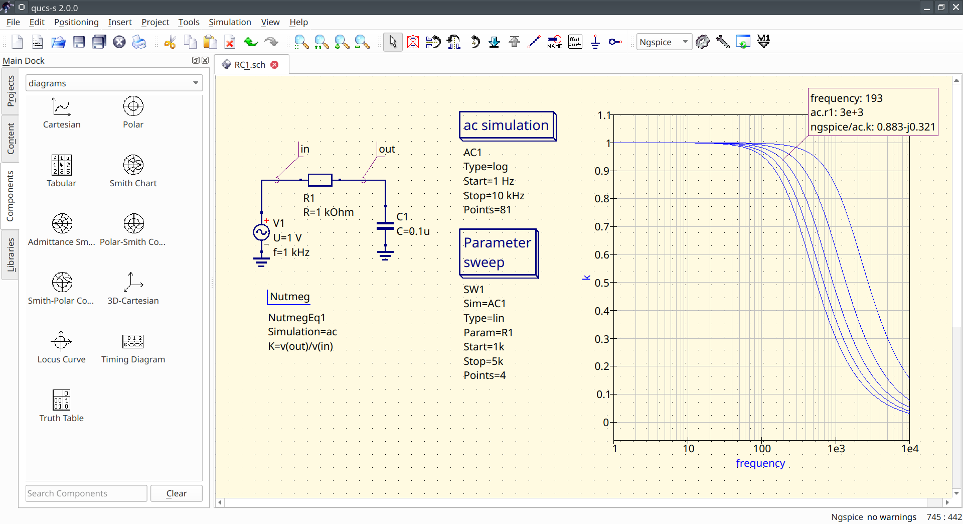
An example of a Nutmeg Equation block being used in a simple RC filter circuit.

Of course, using multiple lines in your Nutmeg Equation block, and using the mathematical functions from the tables above, you can extend the functionality far beyond simple division.